A Nearest neighbor Approach to Estimating Divergence Between Continuous Random Vectors
1. Introduction
The Shannon (or differential) entropy of a continuously distributed random variable (r.v.) X with probability density function (pdf) f is widely used in probability theory and information theory as a measure of uncertainty. It is defined as the negative mean of the logarithm of the density function, i.e.,
k-Nearest neighbor (knn) density estimators were proposed by Mack and Rosenblatt [1]. Penrose and Yukich [2] studied the laws of large numbers for k-nearest neighbor distances. The nearest neighbor entropy estimators when
were studied by Kozachenko and Leonenko [3]. Singh et al. [4] and Leonenko et al. [5] extended these estimators using k-nearest neighbors. Mnatsakanov et al. [6] studied knn entropy estimators for variable rather than fixed k. Eggermontet et al. [7] studied the kernel entropy estimator for univariate smooth distributions. Li et al. [8] studied parametric and nonparametric entropy estimators for univariate multimodal circular distributions. Neeraj et al. [9] studied knn estimators of circular distributions for the data from the Cartesian product, that is,
. Recently, Mnatsakanov et al. [10] proposed an entropy estimator for hyperspherical data based on the moment-recovery (MR) approach (see also Section 4.3).
In this paper, we propose k-nearest neighbor entropy, cross-entropy and KL-divergence estimators for hyperspherical random vectors defined on a unit p-hypersphere
centered at the origin in p-dimensional Euclidean space. Formally,
The surface area
of the hypersphere is well known:
, where Γ is the gamma function. For a part of the hypersphere, the area of a cap with solid angle ϕ relative to its pole is given by Li [11] (cf. Gray [12]):
where sgn is the sign function, and
is the regularized incomplete beta function.
For a random vector from the unit circle
, the von Mises distribution vM
is the most widely used model:
where T is the transpose operator,
and
are the mean direction vector and concentration parameters, and
is the zero-order modified Bessel function of the first kind. Note that the von Mises distribution has a single mode. The multimodal extension to the von Mises distribution is the so-called generalized von Mises model. Its properties are studied by Yfantis and Borgman [13] and Gatto and Jammalamadaka [14].
The generalization of von Mises distribution onto
is the von Mises-Fisher distribution (also known as Langevin distribution) vMF
with pdf,
where the normalization constant is
and
is the ν-order modified Bessel function of the first kind. See Mardia and Jupp [15] (p. 167) for details.
Since von Mises-Fisher distributions are members of the exponential family, by differentiating the cumulant generating function, one can obtain the mean and variance of
:
and
where
, and
. See Watamori [16] for details. Thus the entropy of
is:
and
Spherical distributions have been used to model the orientation distribution functions (ODF) in HARDI (High Angular Resolution Diffusion Imaging). Knutsson [17] proposed a mapping from (
) orientation to a continuous and distance preserving vector space (
). Rieger and Vilet [18] generalized the orientation in any p-dimensional spaces. McGraw et al. [19] used vMF
mixture to model the 3-D ODF and Bhalerao and Westin [20] applied
mixture to 5-D ODF in the mapped space. Entropy of the ODF is proposed as a measure of anisotropy (Özarslan et al. [21], Leow et al. [22]). McGraw et al. [19] used Rényi entropy for the
mixture since it has a closed form. Leow et al. [22] proposed an exponential isotropy measure based on the Shannon entropy. In addition, KL-divergence can be used to measure the closeness of two ODF's. A nonparametric entropy estimator based on knn approach for hyperspherical data provides an easy way to compute the entropy related quantities.
In Section 2, we will propose the knn based entropy estimator for hyperspherical data. The unbiasedness and consistency are proved in this section. In Section 3, the knn estimator is extended to estimate cross entropy and KL-divergence. In Section 4, we present simulation studies using uniform hyperspherical distributions and aforementioned vMF probability models. In addition, the knn entropy estimator is compared with the MR approach proposed in Mnatsakanov et al. [10]. We conclude this study in Section 5.
2. Construction of knn Entropy Estimators
Let
be a random vector having pdf f and
be a set of i.i.d. random vectors drawn from f. To measure the nearness of two vectors x and
, we define a distance measure as the angle between them:
and denote the distance between
and its k-th nearest neighbor in the set of n random vectors by
.
With the distance measure defined above and without loss of generality, the naïve k-nearest neighbor density estimate at
is thus,
where
is the cap area as expressed by (3).
Let
be the natural logarithm of the density estimate at
,
and thus we construct a similar k-nearest neighbor entropy estimator (cf. Singh et al. [4]):
where
is the digamma function.
In the sequel, we shall prove the asymptotic unbiasedness and consistency of
.
2.1. Unbiasedness of
To prove the asymptotic unbiasedness, we first introduce the following lemma:
Lemma 2.1. For a fixed integer , the asymptotic conditional mean of given , is
Proof.
, consider the conditional probability
Equation (11) implies that there are at most k samples falling within the cap
centered at
with area
.
If we let
and
be the number of samples falling onto the cap
, then
, is a binomial random variable. Therefore,
If we let
as
, then
as
. It is reasonable to consider the Poisson approximation of
with mean
. Thus, the limiting distribution of
is a Poisson distribution with mean:
Define a random variable
having the conditional cumulative density function,
then
By taking derivative w.r.t. ℓ, we obtain the conditional pdf of
:
The conditional mean of
is
By change of variable,
,
☐
Corollary 2.2. Given , let , then converges in distribution to , and
Moreover, is a gamma r.v. with the shape parameter k and the rate parameter .
Theorem 2.3. If a pdf f satisfies the following conditions: for some
,
,
, then the estimator proposed in (9) is asymptotically unbiased.
Proof. According to Corollary 2.2 and condition (
), we can show (see (16)–(22)) that for almost all values of
, there exists a positive constant C such that
for all sufficiently large n.
Hence, applying the moment convergence theorem [23] (p. 186), it follows that
for almost all values of
. In addition, using Fatou's lemma and condition (
), we have that
where
is a constant. Therefore,
To show
, one can follow the arguments similar to those used in the proof of Theorem 1 in [24]. Indeed, we can first establish
Namely, we justify that
is valid when
and
. But the inequality
follows immediately from the condition
and
Here
and
is the indicator function.
Now let us denote the distribution function of
by
where
and
is a cap
with the pole x and base radius
. Note also that the functions
(see (3)) and
are both increasing functions.
Now, one can see (cf. (66) in [24]):
where
It is easy to see that for sufficiently large n and almost all
:
and
(cf. (89) and (85) in [24], respectively).
Finally, let us show that
as
. For each x with
, if we choose a
, then for all sufficiently large n,
, since the area of
is equal to
. Using arguments similar to those used in (69)–(72) from [24], we have
The integral in (19) after changing the variable,
, takes the form
since
and
. The first integral in the right side of (20) is bounded as follows:
while for the second one, we have
where
Combination of (15)–(22) and
yields
.
Remark. Note that
where
is the beta function. Hence, in the conditions
, 4, 6 and 8, the difference
can be replaced by
.
2.2. Consistency of
Lemma 2.4. Under the following conditions: for some
,
,
,
the asymptotic variance of is finite and equals , where is the trigamma function.
Proof. The conditions
and
, and the argument similar to the one used in the proof of Theorem 2.3, yields
Therefore, it is sufficient to prove that
. Similarly to (14), we have
Since
,
After some algebra, it can be shown that
☐
Lemma 2.5. For a fixed integer , are asymptotically pairwise independent.
Proof. For a pair of random variables
and
with
and
, following the similar argument for Lemma 2.1,
and
shrink as n increases. Thus, it is safe to assume that
and
are disjoint for large n, and
and
are independent. Hence Lemma 2.5 follows. ☐
Theorem 2.6. Under the conditions through , the variance of decreases with sample size n, that is
and is a consistent estimator of .
Theorem 2.6 can be established by using Theorem 2.3 and Lemmas 2.4 and 2.5, and
For a finite sample, the variance of
can be approximated by
. For instance, for the uniform distribution,
and
and for a vMF
,
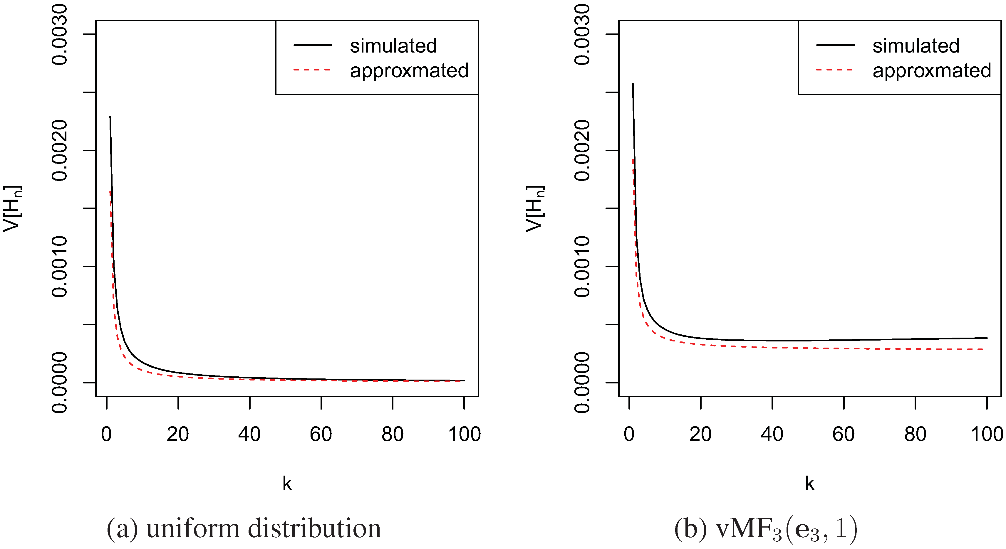
. See the illustration in Figure 1. The simulation was done with sample size
and the number of simulations was
. Since
is a decreasing function, the variance of
decreases when k increases.
Figure 1. Variances of
by simulation and approximation.
Figure 1. Variances of
by simulation and approximation.
3. Estimation of Cross Entropy and KL-divergence
3.1. Estimation of Cross Entropy
The definition of cross entropy between continuous pdf's f and g is,
Given a random sample of size n from f, {
}, and a random sample of size m from g, {
}, on a hypersphere, denote the knn density estimator of g by
. Similarly to (7),
where
is the distance from
to its k-th nearest neighbor in {
}. Analogously to the entropy estimator (9), the cross entropy can be estimated by:
Under the conditions
–
, for a fixed integer
, one can show that
is asymptotically unbiased. Moreover, by similar reasoning applied for
, one can show that
is also consistent and
. For example, when both f and g are vMF with the same mean direction and different concentration parameters,
and
, respectively, the approximate variance will be
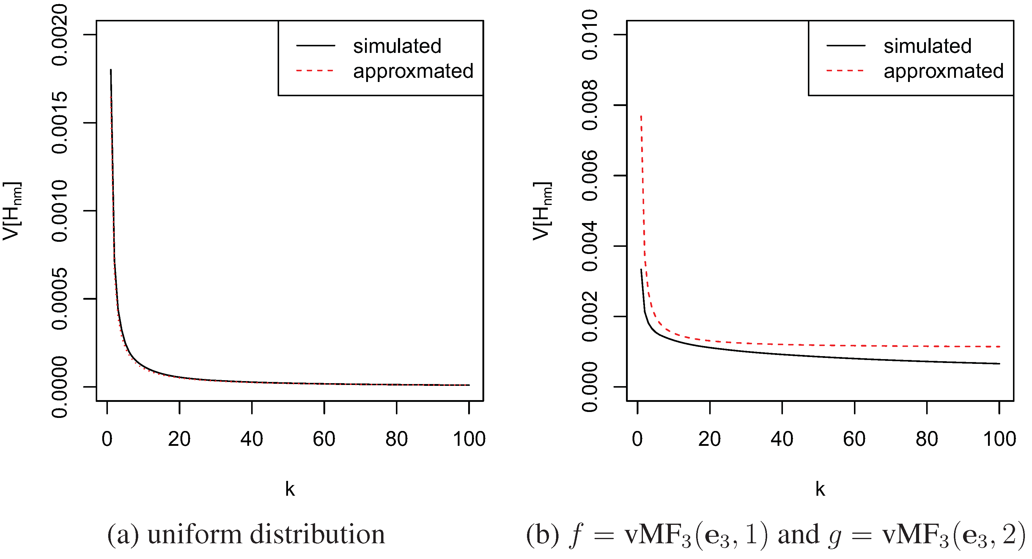
. Figure 2 shows the approximated and simulated variance of the knn estimators for cross entropy are close to each other and both decrease with k. The simulation is done with sample size
and the number of simulations was
.
Figure 2. Variances of
by simulation and approximation.
Figure 2. Variances of
by simulation and approximation.
3.2. Estimation of KL-Divergence
KL-divergence is also known as relative entropy. It is used to measure the similarity of two distributions. Wang et al. [24] studied the knn estimator of KL-divergence for distributions defined on
. Here we propose the knn estimator of KL-divergence of continuous distribution f from g defined on a hypersphere. The KL-divergence is defined as:
Equation (30) can also be expressed as
. Then the knn estimator of KL-divergence is constructed as
, i.e.,
where
is defined as in (28). Besides, for finite samples, the variance of the estimator,
, is approximately
. When f and g are vMF as mentioned above, with concentration parameter
and
, respectively, we have:
and
So the approximate variance is
. Figure 3 shows the approximated and simulated variance of the knn estimators for KL-divergence. The approximation for von Mises-Fisher distribution is not as good as the one for uniform distributions. This could be due to the modality of von Mises-Fisher distributions or the finitude of sample sizes. The larger the sample size, the closer the approximation is to the true value.
Figure 3. Variances of
by simulation and approximation.
Figure 3. Variances of
by simulation and approximation.

In summary, we have
Corollary 3.1. (1) Under conditions and for some ,
,
,
for a fixed integer , the knn estimator of KL-divergence given in (31) is asymptotically unbiased.
(2) Under condition and for some ,
,
,
for a fixed integer , the knn estimator of KL-divergence given in (31) is asymptotically consistent.
To prove the last two corollaries, one can follow the similar steps proposed in Wang et al. [24].
4. Simulation Study
To demonstrate the proposed knn entropy estimators and assess their performance for finite samples, we conducted simulations for the uniform distribution and von Mises-Fisher distributions with the p-coordinate unit vector,
, as the common mean direction for
and 10. For each distribution, we drew samples of size
, 500 and 1000. All simulations were repeated
times. Bias, standard deviation (SD) and root mean squared error (RMSE) were calculated.
4.1. Bias and Standard Deviation
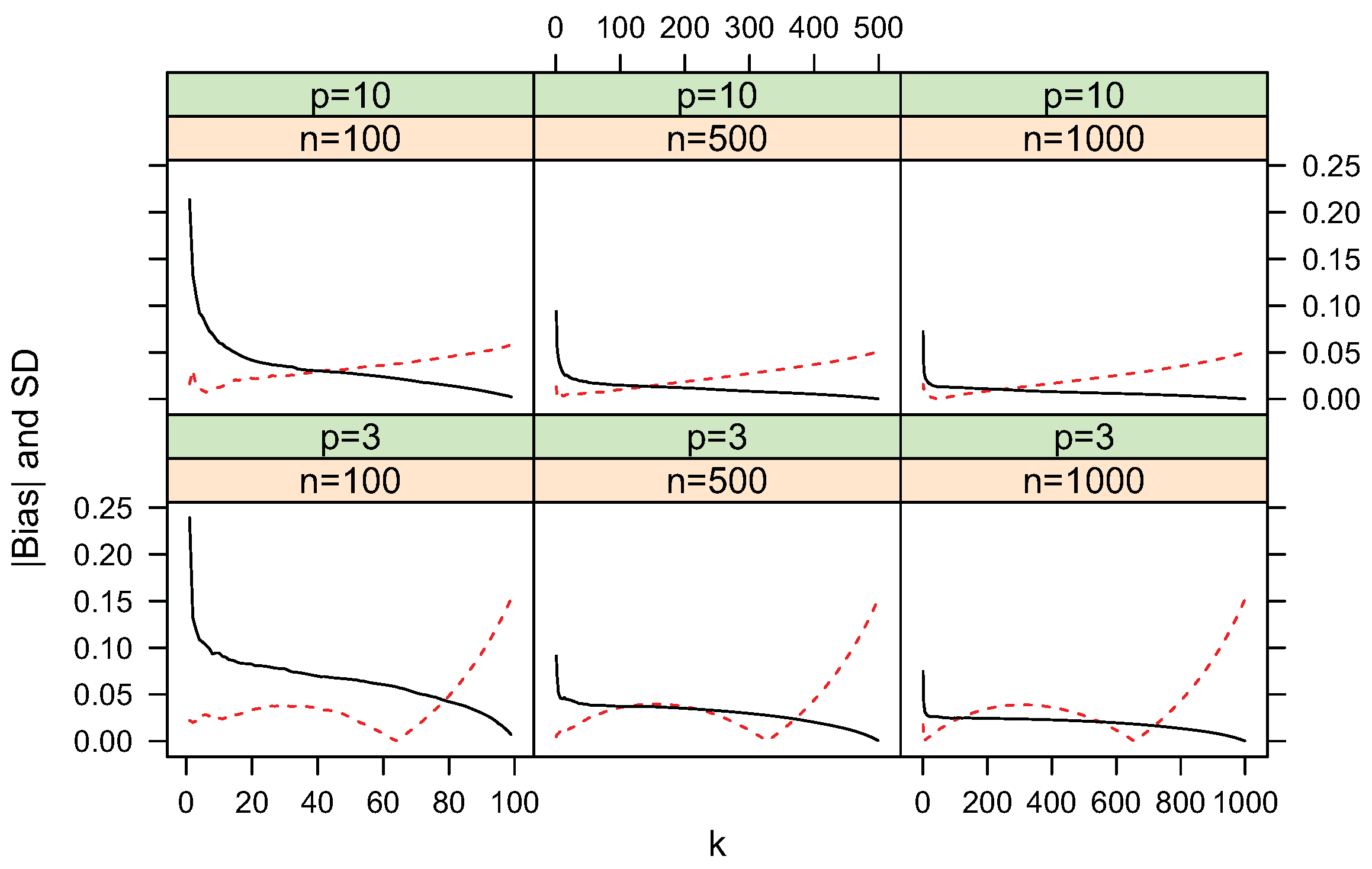
Figure 4, Figure 5, Figure 6, Figure 7, Figure 8 and Figure 9 show simulated bias and standard deviation of the proposed entropy, cross-entropy and KL-divergence estimators along different k. The pattern for the standard deviation is clear. It decreases sharply then slowly as k increases. This is consistent with the variance approximations described in Section 2 and Section 3. The pattern for bias is diverse. For uniform distributions, the bias term is very small. When the underlying distribution has a mode, for example, vMF models used in the current simulations, the relation between bias and k becomes complex and the bias term can be larger for larger k values.
Figure 4.
(dashed line) and standard deviation (solid line) of entropy estimate
for uniform distributions.
Figure 4.
(dashed line) and standard deviation (solid line) of entropy estimate
for uniform distributions.

Figure 5.
(dashed line) and standard deviation (solid line) of entropy estimate
for vMF
distributions.
Figure 5.
(dashed line) and standard deviation (solid line) of entropy estimate
for vMF
distributions.
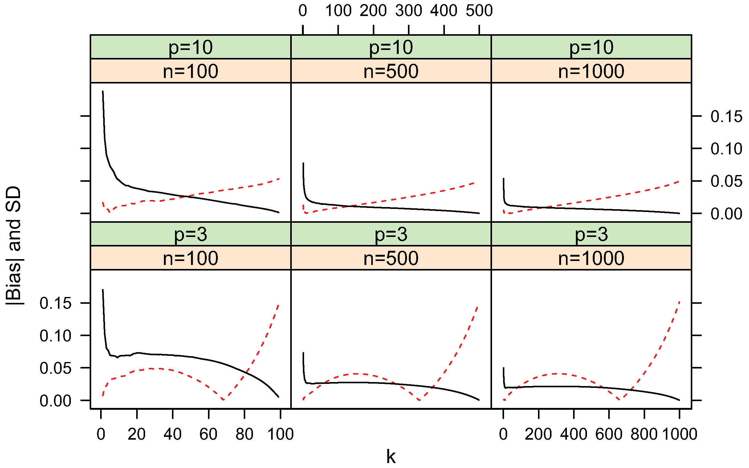
Figure 6.
(dashed line) and standard deviation (solid line) of cross entropy estimate
for uniform distributions.
Figure 6.
(dashed line) and standard deviation (solid line) of cross entropy estimate
for uniform distributions.
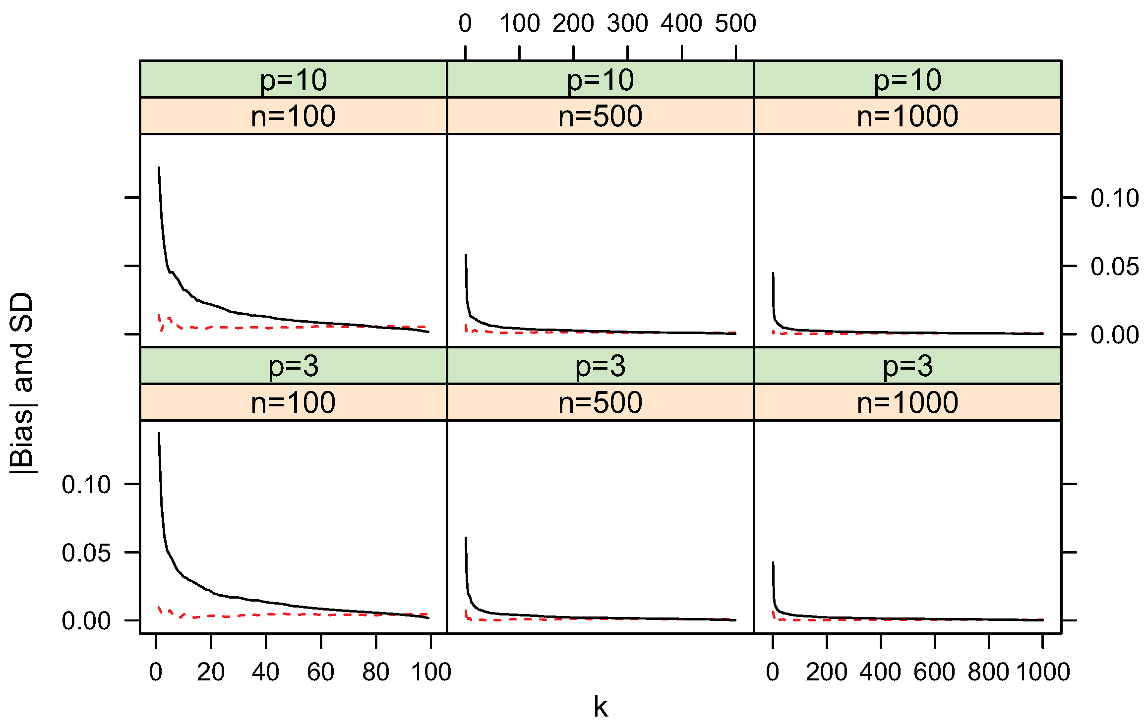
Figure 7.
(dashed line) and standard deviation (solid line) of cross entropy estimate
for
and
uniform distributions.
Figure 7.
(dashed line) and standard deviation (solid line) of cross entropy estimate
for
and
uniform distributions.
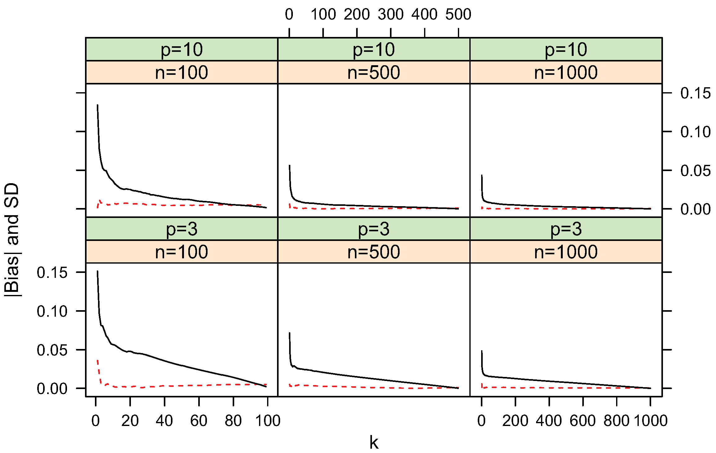
Figure 8.
(dashed line) and standard deviation (solid line) of KL-divergence estimate
for uniform distributions.
Figure 8.
(dashed line) and standard deviation (solid line) of KL-divergence estimate
for uniform distributions.

Figure 9.
(dashed line) and standard deviation (solid line) of KL-divergence estimate
for
and
uniform distributions.
Figure 9.
(dashed line) and standard deviation (solid line) of KL-divergence estimate
for
and
uniform distributions.
4.2. Convergence
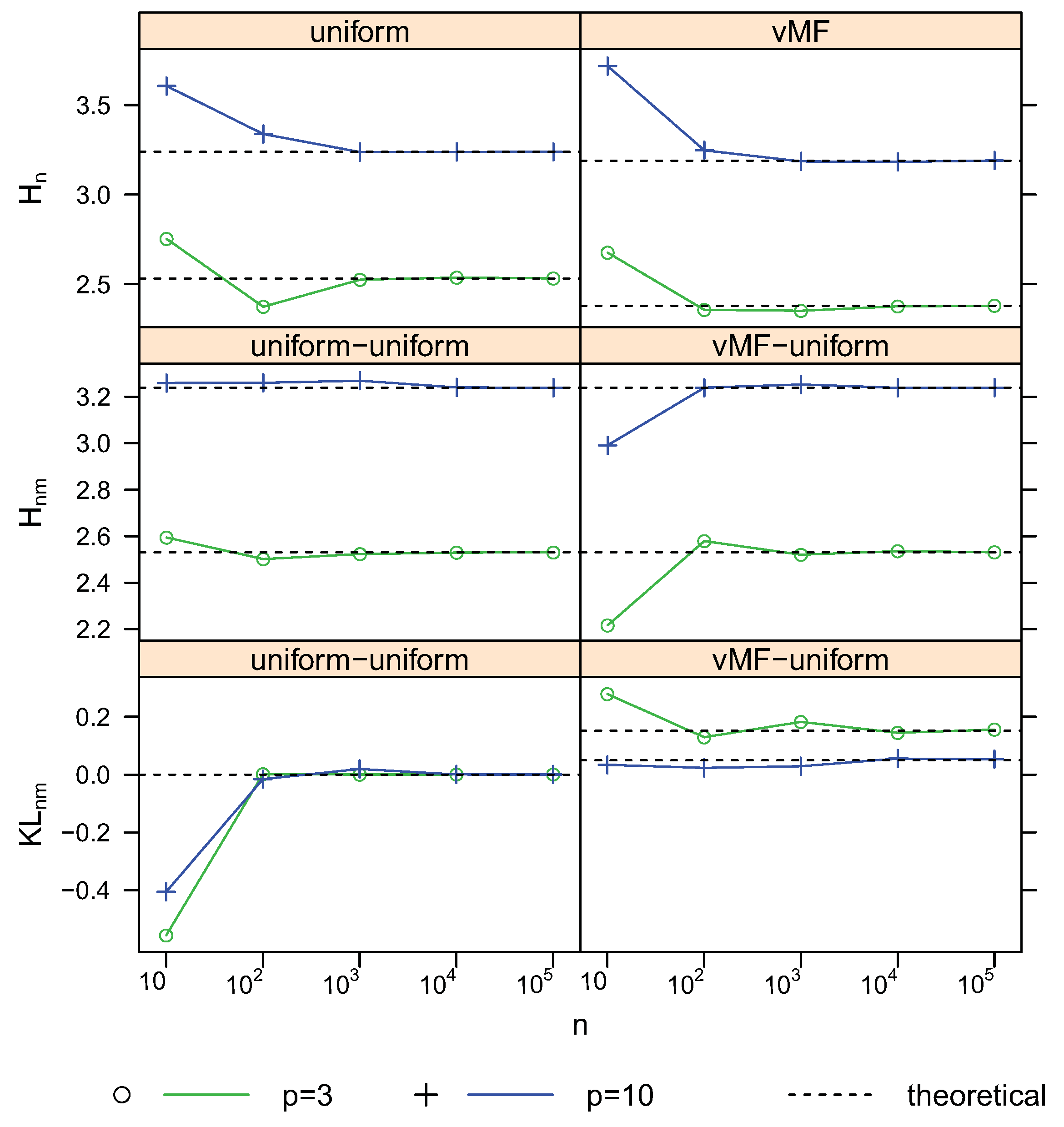
To validate the consistency, we conducted simulations of different sample size n from 10 to 100,000 for the distribution models used above. Figure 10 and Figure 11 shows the estimates and theoretical values of entropy, cross-entropy and KL-divergence for different sample sizes with
and
2–12, respectively. The proposed estimators converge to the corresponding theoretical values quickly. Thus the consistency of these estimators are verified. The choice of k is an open problem for knn based estimation approaches. These figures show that using lager k, e.g., the logarithm of n, for lager n, is giving a slightly better preference.
Figure 10. Convergence of estimates with sample size n using the first nearest neighbor. For vMF
,
.
Figure 10. Convergence of estimates with sample size n using the first nearest neighbor. For vMF
,
.
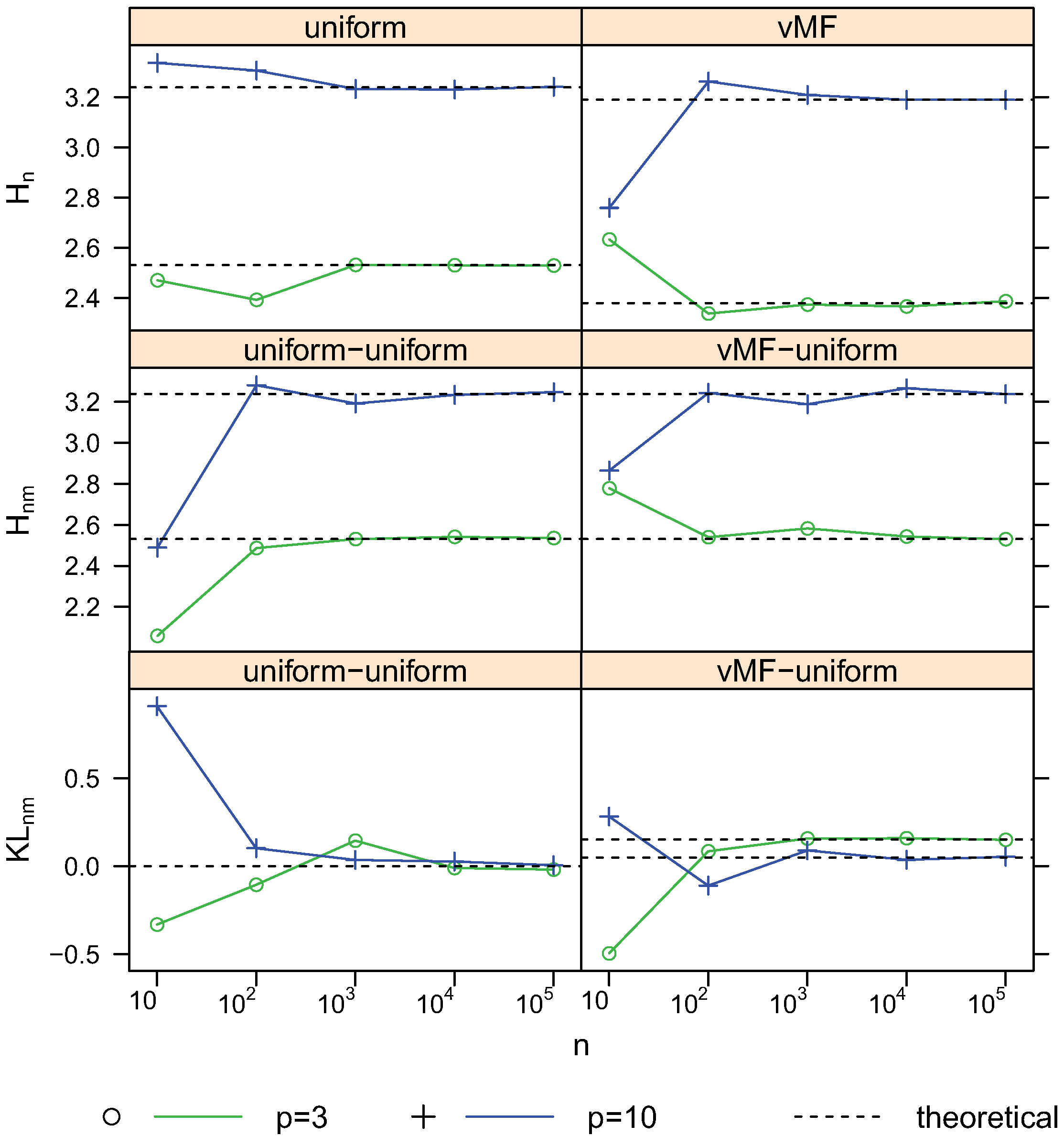
Figure 11. Convergence of estimates with sample size n using
nearest neighbors. For vMF
,
.
Figure 11. Convergence of estimates with sample size n using
nearest neighbors. For vMF
,
.
4.3. Comparison with the Moment-Recovered Construction
Another entropy estimator for hyperspherical data was developed recently by Mnatsakanov et al. [10] using MR approach. We call this estimator the MR entropy estimator and denote it by
:
where
is the estimated probability of the cap
defined by the revolution axis
and t is the distance from the cap base to the origin and acts as a tuning parameter. Namely, (see Mnatsakanov et al. [10]),
Via simulation study, the empirical comparison between
and
was done for the uniform and vMF distributions. The results are presented in Table 1. The values of k and t listed in the table are the optimal ones in the sense of minimizing RMSE. Z-tests and F-tests (at
) were performed to compare the bias, standard deviation (variance) and RMSE (MSE) between the knn estimators and corresponding MR estimators. In general, for uniform distributions, there are no significant difference for biases. Among other comparisons, the differences are significant. Specifically, knn achieves slightly smaller bias and RMSE values than those of the MR method. The standard deviations of knn method are also smaller for the uniform distribution but larger for vMF distributions than those based on MR approach.
Table 1. Comparison of knn and moment methods by simulations for spherical distributions.
| Method | knn | MR | |||||||
|---|---|---|---|---|---|---|---|---|---|
| p | n | k | bias | SD | RMSE | t | bias | SD | RMSE |
| Uniform: | |||||||||
| 3 | 100 | 99 | 0.00500 | 0.00147 | 0.00521 | 0.01 | 0.00523 | 0.01188 | 0.01298 |
| 3 | 500 | 499 | 0.00100 | 0.00013 | 0.00101 | 0.01 | 0.00107 | 0.00233 | 0.00257 |
| 3 | 1000 | 999 | 0.00050 | 0.00005 | 0.00050 | 0.01 | 0.00051 | 0.00120 | 0.00130 |
| 10 | 100 | 99 | 0.00503 | 0.00130 | 0.00520 | 0.01 | 0.00528 | 0.01331 | 0.01432 |
| 10 | 500 | 499 | 0.00100 | 0.00011 | 0.00101 | 0.01 | 0.00102 | 0.00264 | 0.00283 |
| 10 | 1000 | 999 | 0.00050 | 0.00004 | 0.00050 | 0.01 | 0.00052 | 0.00130 | 0.00140 |
| vMF: | |||||||||
| 3 | 100 | 71 | 0.01697 | 0.05142 | 0.05415 | 0.30 | 0.02929 | 0.04702 | 0.05540 |
| 3 | 500 | 337 | 0.00310 | 0.02336 | 0.02356 | 0.66 | 0.00969 | 0.02318 | 0.02512 |
| 3 | 1000 | 670 | 0.00145 | 0.01662 | 0.01668 | 0.74 | 0.00620 | 0.01658 | 0.01770 |
| 10 | 100 | 46 | 0.02395 | 0.02567 | 0.03511 | 0.12 | 0.02895 | 0.02363 | 0.03737 |
| 10 | 500 | 76 | 0.00702 | 0.01361 | 0.01531 | 0.40 | 0.01407 | 0.01247 | 0.01881 |
| 10 | 1000 | 90 | 0.00366 | 0.01026 | 0.01089 | 0.47 | 0.01115 | 0.00907 | 0.01437 |
5. Discussion and Conclusions
In this paper, the knn based estimators for entropy, cross-entropy and Kullback-Leibler divergence are proposed for distributions on hyperspheres. Asymptotic properties such as unbiasedness and consistency are proved and validated by simulation studies using uniform and von Mises-Fisher distribution models. The variances of these estimators decrease with k. For uniform distributions, variance is dominant and bias is negligible. When the underlying distributions are modal, the bias can be large if k is large. In general, we conclude that the behavior of knn and MR entropy estimators have similar performance in terms of root mean square error.
Acknowledgements and Disclaimer
The authors thank the anonymous referees for their helpful comments and suggestions. The research of Robert Mnatsakanov was supported by NSF grant DMS-0906639. The findings and conclusions in this report are those of the author(s) and do not necessarily represent the views of the National Institute for Occupational Safety and Health.
Source: https://www.mdpi.com/1099-4300/13/3/650/htm
0 Response to "A Nearest neighbor Approach to Estimating Divergence Between Continuous Random Vectors"
Post a Comment